Sort and filter data

Sort Data

You can quickly sort your data in a spreadsheet using one of the available options:

• Ascending is used to sort your data in ascending order - A to Z alphabetically or smallest to largest for numerical data.
• Descending is used to sort your data in descending order - Z to A alphabetically or largest to smallest for numerical data.

Note: the Sort options are accessible from both Home and Data tab.

To sort your data,

1. select a range of cells you wish to sort (you can select a single cell in a range to sort the entire range),
2. click the Sort ascending
   icon situated at the Home or Data tab of the top toolbar to sort your data in ascending order,
   OR
   click the Sort descending
   icon situated at the Home or Data tab of the top toolbar to sort your data in descending order.

Note: if you select a single column/row within a cell range or a part of the column/row, you will be asked if you want to expand the selection to include adjacent cells or sort the selected data only.

You can also sort your data using the contextual menu options. Right-click the selected range of cells, select the Sort option from the menu and then select Ascending or Descending option from the submenu.

It's also possible to sort the data by a color using the contextual menu:

1. right-click a cell containing the color you want to sort your data by,
2. select the Sort option from the menu,
3. select the necessary option from the submenu:
   • Selected Cell Color on top - to display the entries with the same cell background color on the top of the column,
   • Selected Font Color on top - to display the entries with the same font color on the top of the column.

Filter Data

To display only the rows that meet certain criteria and hide other ones, make use of the Filter option.

Note: the Filter options are accessible from both Home and Data tab.

To enable a filter,

1. Select a range of cells containing data to filter (you can select a single cell in a range to filter the entire range),
2. Click the Filter
   icon situated at the Home or Data tab of the top toolbar.

   The drop-down arrow will appear in the first cell of each column of the selected cell range. It means that the filter is enabled.

To apply a filter,

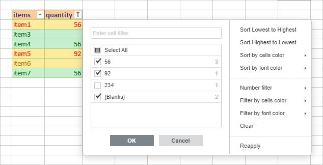
1. Click the drop-down arrow
   . The Filter option list will open:

   

   Note: you can adjust the filter window size by dragging its right border to the right or to the left to display the data as convenient as possible.

2. Adjust the filter parameters. You can proceed in one of the following three ways: select the data to display, filter data by certain criteria or filter data by color.

   • Select the data to display

     Uncheck the boxes near the data you need to hide. For your convenience all the data wintin the Filter option list are sorted in ascending order.

     The number of unique values in the filtered range is displayed to the right of each value within the filter window.

     Note: the {Blanks} check box corresponds to the empty cells. It is available if the selected range of cells contains at least one empty cell.

     To facilitate the process make use of the search field on the top. Enter your query, entirely or partially, in the field - the values that include these characters will be displayed in the list below. The following two options will also be available:

     • Select All Search Results - is checked by default. It allows to select all the values that correspond to your query in the list.
     • Add current selection to filter - if you check this box, the selected values will not be hidden when you apply the filter.

     After you select all the necessary data, click the OK button in the Filter option list to apply the filter.

   • Filter data by certain criteria

     Depending on the data contained in the selected column, you can choose either the Number filter or the Text filter option in the right part of the Filter options list, and then select one of the options from the submenu:

     • For the Number filter the following options are available: Equals..., Does not equal..., Greater than..., Greater than or equal to..., Less than..., Less than or equal to..., Between, Top 10, Above Average, Below Average, Custom Filter....
     • For the Text filter the following options are available: Equals..., Does not equal..., Begins with..., Does not begin with..., Ends with..., Does not end with..., Contains..., Does not contain..., Custom Filter....

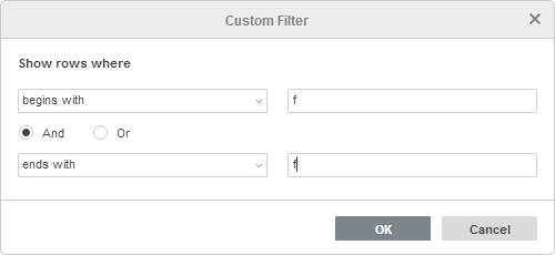
     After you select one of the above options (apart from the Top 10 and Above/Below Average ones), the Custom Filter window will open. The corresponding criterion will be selected in the upper drop-down list. Enter the necessary value in the field on the right.

     To add one more criterion, use the And radiobutton if you need the data to satisfy both criteria or click the Or radiobutton if either or both criteria can be satisfied. Then select the second criterion from the lower drop-down list and enter the necessary value on the right.

     Click OK to apply the filter.

     

     If you choose the Custom Filter... option from the Number/Text filter option list, the first criterion is not selected automatically, you can set it yourself.

     If you choose the Top 10 option from the Number filter option list, a new window will open:

     

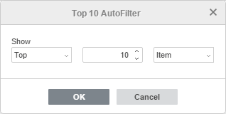
     The first drop-down list allows to choose if you wish to display the highest (Top) or lowest (Bottom) values. The second field allows to specify how many entries from the list or which percent of the overall entries number you want to display (you can enter a number from 1 to 500). The third drop-down list allows to set units of measure: Item or Percent. Once the necessary parameters are set, click OK to apply the filter.

     If you choose the Above/Below Average option from the Number filter option list, the filter will be applied right now.

   • Filter data by color

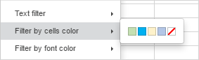
     If the cell range you want to filter contains some cells you have formatted changing their background or font color (manually or using predefined styles), you can use one of the following options:

     • Filter by cells color - to display only the entries with a certain cell background color and hide other ones,
     • Filter by font color - to display only the entries with a certain cell font color and hide other ones.

     When you select the necessary option, a palette that contains colors used in the selected cell range will open. Choose one of the colors to apply the filter.

     

   The Filter button will appear in the first cell of the column. It means that the filter is applied. The number of filtered records will be displayed at the status bar (e.g. 25 of 80 records filtered).

   Note: when the filter is applied, the rows that are filtered out cannot be modified when autofilling, formatting, deleting the visible contents. Such actions affect the visible rows only, the rows that are hidden by the filter remain unchanged. When copying and pasting the filtered data, only visible rows can be copied and pasted. This is not equivalent to manually hidden rows which are affected by all similar actions.

Sort filtered data

You can set the sorting order of the data you have enabled or applied filter for. Click the drop-down arrow or the Filter button and select one of the options in the Filter option list:

• Sort Lowest to Highest - allows to sort your data in ascending order, displaying the lowest value on the top of the column,
• Sort Highest to Lowest - allows to sort your data in descending order, displaying the highest value on the top of the column,
• Sort by cells color - allows to select one of the colors and display the entries with the same cell background color on the top of the column,
• Sort by font color - allows to select one of the colors and display the entries with the same font color on the top of the column.

The latter two options can be used if the cell range you want to sort contains some cells you have formatted changing their background or font color (manually or using predefined styles).

The sorting direction will be indicated by an arrow in the filter buttons.

• if the data is sorted in ascending order, the drop-down arrow in the first cell of the column looks like this:
  and the Filter button looks the following way:
  .
• if the data is sorted in descending order, the drop-down arrow in the first cell of the column looks like this:
  and the Filter button looks the following way:
  .

You can also quickly sort the data by a color using the contextual menu options:

1. right-click a cell containing the color you want to sort your data by,
2. select the Sort option from the menu,
3. select the necessary option from the submenu:
   • Selected Cell Color on top - to display the entries with the same cell background color on the top of the column,
   • Selected Font Color on top - to display the entries with the same font color on the top of the column.

Filter by the selected cell contents

You can also quickly filter your data by the selected cell contents using the contextual menu options. Right-click a cell, select the Filter option from the menu and then select one of the available options:

• Filter by Selected cell's value - to display only the entries with the same value as the selected cell contains.
• Filter by cell's color - to display only the entries with the same cell background color as the selected cell has.
• Filter by font color - to display only the entries with the same cell font color as the selected cell has.

Format as Table Template

To facilitate the work with your data Spreadsheet Editor allows you to apply a table template to a selected cell range automatically enabling the filter. To do that,

1. select a range of cells you need to format,
2. click the Format as table template
   icon situated at the Home tab of the top toolbar.
3. select the template you need in the gallery,
4. in the opened pop-up window check the range of cells to be formatted as a table,
5. check the Title if you wish the table headers to be included in the selected range of cells, otherwise the header row will be added at the top while the selected range of cells will be moved one row down,
6. click the OK button to apply the selected template.

The template will be applied to the selected range of cells and you will be able to edit the table headers and apply the filter to work with your data.

It's also possible to insert a formatted table using the Table button at the Insert tab. In this case, the default table template is applied.

Note: once you create a new formatted table, a default name (Table1, Table2 etc.) will be automatically assigned to the table. You can change this name making it more meaningful and use it for further work.

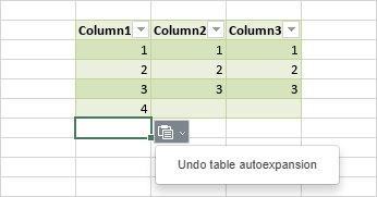
If you enter a new value in a cell below the table last row (if the table does not have the Total row) or in a cell to the right of the table last column, the formatted table will be automatically extended to include a new row or column. If you do not want to expand the table, click the button that appears and select the Undo table autoexpansion option. Once you undo this action, the Redo table autoexpansion option will be available in this menu.

Some of the table settings can be altered using the Table settings tab of the right sidebar that opens if you select at least one cell within the table with the mouse and click the Table settings icon on the right.

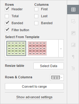
The Rows and Columns sections on the top allow you to emphasize certain rows/columns applying a specific formatting to them, or highlight different rows/columns with the different background colors to clearly distinguish them. The following options are available:

• Header - allows to display the header row.
• Total - adds the Summary row at the bottom of the table.
• Banded - enables the background color alternation for odd and even rows.
• Filter button - allows to display the drop-down arrows
  in the header row cells. This option is only available when the Header option is selected.
• First - emphasizes the leftmost column in the table with a special formatting.
• Last - emphasizes the rightmost column in the table with a special formatting.
• Banded - enables the background color alternation for odd and even columns.

The Select From Template section allows you to choose one of the predefined tables styles. Each template combines certain formatting parameters, such as a background color, border style, row/column banding etc. Depending on the options checked in the Rows and/or Columns sections above, the templates set will be displayed differently. For example, if you've checked the Header option in the Rows section and the Banded option in the Columns section, the displayed templates list will include only templates with the header row and banded columns enabled:

If you want to clear the current table style (background color, borders etc.) without removing the table itself, apply the None template from the template list:

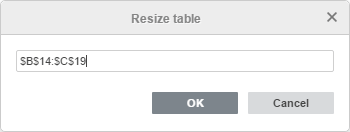
The Resize table section allows you to change the cell range the table formatting is applied to. Click the Select Data button - a new pop-up window will open. Change the link to the cell range in the entry field or select the necessary cell range on the worksheet with the mouse and click the OK button.

The Rows & Columns section allows you to perform the following operations:

• Select a row, column, all columns data excluding the header row, or the entire table including the header row.
• Insert a new row above or below the selected one as well as a new column to the left or to the right of the selected one.
• Delete a row, column (depending on the cursor position or the selection), or the entire table.

Note: the options of the Rows & Columns section are also accessible from the right-click menu.

The Convert to range button can be used if you want to transform the table into a regular data range removing the filter but preserving the table style (i.e. cell and font colors etc.). Once you apply this option, the Table settings tab at the right sidebar will be unavailable.

To change the advanced table properties, use the Show advanced settings link at the right sidebar. The table properties window will open:

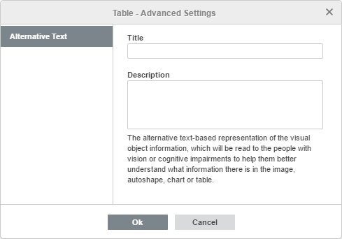
The Alternative Text tab allows to specify a Title and Description which will be read to the people with vision or cognitive impairments to help them better understand what information there is in the table.

Reapply Filter

If the filtered data has been changed, you can refresh the filter to display an up-to-date result:

1. click the Filter
   button in the first cell of the column that contains the filtered data,
2. select the Reapply option in the Filter option list that opens.

You can also right-click a cell within the column that contains the filtered data and select the Reapply option from the contextual menu.

Clear Filter

To clear the filter,

1. click the Filter
   button in the first cell of the column that contains the filtered data,
2. select the Clear option in the Filter option list that opens.

You can also proceed in the following way:

1. select the range of cells containing the filtered data,
2. click the Clear filter
   icon situated at the Home or Data tab of the top toolbar.

The filter will remain enabled, but all the applied filter parameters will be removed, and the Filter buttons in the first cells of the columns will change into the drop-down arrows .

Remove Filter

To remove the filter,

1. select the range of cells containing the filtered data,
2. click the Filter
   icon situated at the Home or Data tab of the top toolbar.

The filter will be disabled, and the drop-down arrows will disappear from the first cells of the columns.

Sort data by several columns/rows

To sort data by several columns/rows you can create several sorting levels using the Custom Sort function.

1. select a range of cells you wish to sort (you can select a single cell in a range to sort the entire range),
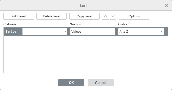
2. click the Custom Sort
   icon situated at the Data tab of the top toolbar,
3. the Sort window opens. Sorting by columns is selected by default.

   

   To change sort orientation (i.e. sort data by rows instead of columns) click the Options button on the top. The Sort Options window will open:

   

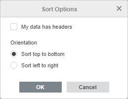
   1. check the My data has headers box, if necessary,
   2. choose the necessary Orientation: Sort top to bottom to sort data by columns or Sort left to right to sort data by rows,
   3. click OK to apply the changes and close the window.
4. set the first sorting level in the Sort by field:

   

   • in the Column / Row section, select the first column / row you want to sort,
   • in the Sort on list choose one of the following options: Values, Cell color, or Font color,
   • in the Order list, specify the necessary sorting order. The available options differ depending on the option chosen in the Sort on list:
     • if the Values option is selected, choose the Ascending / Descending option if the cell range contains numbers or A to Z / Z to A option if the cell range contains text values,
     • if the Cell color option is selected, choose the necessary cell color and select the Top / Below option for columns or Left / Right option for rows,
     • if the Font color option is selected, choose the necessary font color and select the Top / Below option for columns or Left / Right option for rows.
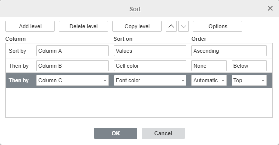
5. add the next sorting level by clicking the Add level button, select the second column / row you want to sort and specify other sorting parameters in the Then by field as described above. If necessary, add more levels in the same way.
6. manage the added levels using the buttons at the top of the window: Delete level, Copy level or change the level order by using the arrow buttons Move the level up / Move the level down,
7. click OK to apply the changes and close the window.

The data will be sorted according to the specified sorting levels.

Alla pagina precedente