Use formatted tables

Create a new formatted table

To make it easier for you to work with data, the Spreadsheet Editor allows you to apply a table template to the selected cell range and automatically enable the filter. To do that,

1. select a range of cells you need to format,
2. click the Format as table template
   icon situated on the Home tab of the top toolbar,
3. select the required template in the gallery,
4. in the opened pop-up window, check the cell range to be formatted as a table,
5. check the Title if you wish the table headers to be included in the selected cell range, otherwise, the header row will be added at the top while the selected cell range will be moved one row down,
6. click the OK button to apply the selected template.

The template will be applied to the selected range of cells, and you will be able to edit the table headers and apply the filter to work with your data.

It's also possible to insert a formatted table using the Table button on the Insert tab. In this case, the default table template is applied.

Note: once you create a new formatted table, the default name (Table1, Table2, etc.) will be automatically assigned to the table. You can change this name making it more meaningful and use it for further work.

If you enter a new value in the cell below the last row of the table (if the table does not have the Total row) or in the cell to the right of the last column of the table, the formatted table will be automatically extended to include a new row or column. If you do not want to expand the table, click the Paste special button that will appear and select the Undo table autoexpansion option. Once you undo this action, the Redo table autoexpansion option will be available in this menu.

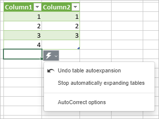
Note: To enable/disable table auto-expansion, select the Stop automatically expanding tables option in the Paste special button menu or go to Advanced Settings -> Spell Checking -> Proofing -> AutoCorrect Options -> AutoFormat As You Type.

Select rows and columns

To select an entire row in the formatted table, move the mouse cursor over the left border of the table row until it turns into the black arrow , then left-click.

To select an entire column in the formatted table, move the mouse cursor over the top edge of the column header until it turns into the black arrow , then left-click. If you click once, the column data will be selected (as it is shown on the image below); if you click twice, the entire column including the header will be selected.

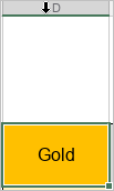
To select an entire formatted table, move the mouse cursor over the upper left corner of the formatted table until it turns into the diagonal black arrow , then left-click.

Edit formatted tables

Some of the table settings can be changed using the Table settings tab of the right sidebar that will open if you select at least one cell within the table with the mouse and click the Table settings icon on the right.

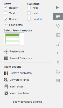
The Rows and Columns sections on the top allow you to emphasize certain rows/columns applying specific formatting to them, or highlight different rows/columns with different background colors to clearly distinguish them. The following options are available:

• Header - allows you to display the header row.
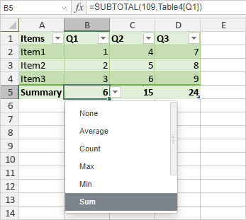
• Total - adds the Summary row at the bottom of the table.

  Note: if this option is selected, you can also select a function to calculate the summary values. Once you select a cell in the Summary row, the button will be available to the right of the cell. Click it and choose the necessary function from the list: Average, Count, Max, Min, Sum, StdDev, or Var. The More functions option allows you to open the Insert Function window and choose any other function. If you choose the None option, the currently selected cell in the Summary row will not display a summary value for this column.

  

• Banded - enables the background color alternation for odd and even rows.
• Filter button - allows you to display the drop-down arrows
  in each cell of the header row. This option is only available when the Header option is selected.
• First - emphasizes the leftmost column in the table with special formatting.
• Last - emphasizes the rightmost column in the table with special formatting.
• Banded - enables the background color alternation for odd and even columns.

The Select From Template section allows you to choose one of the predefined tables styles. Each template combines certain formatting parameters, such as a background color, border style, row/column banding, etc. Depending on the options checked in the Rows and/or Columns sections above, the templates set will be displayed differently. For example, if you've checked the Header option in the Rows section and the Banded option in the Columns section, the displayed templates list will include only templates with the header row and banded columns enabled:

If you want to remove the current table style (background color, borders, etc.) without removing the table itself, apply the None template from the template list:

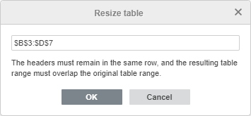
The Resize table section allows you to change the cell range the table formatting is applied to. Click the Select Data button - a new pop-up window will open. Change the link to the cell range in the entry field or select the necessary cell range in the worksheet with the mouse and click the OK button.

Note: The headers must remain in the same row, and the resulting table range must overlap the original table range.

The Rows & Columns section allows you to perform the following operations:

• Select a row, column, all columns data excluding the header row, or the entire table including the header row.
• Insert a new row above or below the selected one as well as a new column to the left or the right of the selected one.
• Delete a row, column (depending on the cursor position or the selection), or the entire table.

Note: the options of the Rows & Columns section are also accessible from the right-click menu.

The Remove duplicates option can be used if you want to remove duplicate values from the formatted table. For more details on removing duplicates, please refer to this page.

The Convert to range option can be used if you want to transform the table into a regular data range removing the filter but preserving the table style (i.e. cell and font colors, etc.). Once you apply this option, the Table settings tab on the right sidebar will be unavailable.

The Insert slicer option is used to create a slicer for the formatted table. For more details on working with slicers, please refer to this page.

The Insert pivot table option is used to create a pivot table on the base of the formatted table. For more details on working with pivot tables, please refer to this page.

Adjust formatted table advanced settings

To change the advanced table properties, use the Show advanced settings link on the right sidebar. The 'Table - Advanced Settings' window will open:

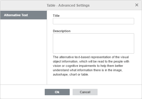
The Alternative Text tab allows you to specify the Title and the Description which will be read to people with vision or cognitive impairments to help them better understand what information the table contains.

Note: To enable/disable table auto-expansion, go to Advanced Settings -> Spell Checking -> Proofing -> AutoCorrect Options -> AutoFormat As You Type.

Use Formula Autocomplete to Add Formulas to Formatted Tables

The Formula Autocomplete list displays all the available options when you apply formulas to formatted tables. You can add a reference to a table in your formula inside or outside a table. Columns and item names are used instead of cell addresses as references.

The example below shows a reference to a table in the SUM function.

1. Select a cell and start typing a formula beginning with an equal sign, select the necessary function from the Formula Autocomplete list. After the opening parenthesis, start typing the table name, and select the appropriate name from the Formula Autocomplete list.

   

2. Then type an opening bracket [ to open the drop-down list that contains columns and items that can be used in the formula. A tooltip describing the reference appears when you hover the mouse pointer over it in the list.

   

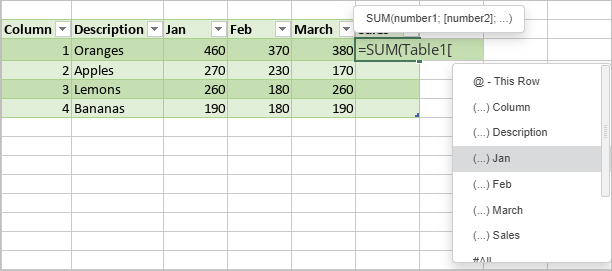
Note: Each reference must contain an opening and a closing bracket. Don’t forget to check formula syntax.

Return to previous page