Create and edit pivot tables
Pivot tables allow you to group and arrange data of large data sets to get summarized information. In the Spreadsheet Editor you can reorganize data in many different ways to display only the necessary information and focus on important aspects.
Create a new pivot table
To create a pivot table,
- Prepare the source data set you want to use for creating a pivot table. It should include column headers. The data set should not contain empty rows or columns.
- Select any cell within the source data range.
-
Switch to the Pivot Table tab of the top toolbar and click the Insert Table icon.
If you want to create a pivot table on the base of a formatted table, you can also use the Insert pivot table option on the Table settings tab of the right sidebar.
-
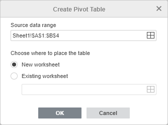
The Create Pivot Table window will appear.
-
The Source data range is already specified. In this case, all data from the source data range will be used. If you want to change the data range (e.g. to include only a part of source data), click the icon. In the Select Data Range window, enter the necessary data range in the following format: Sheet1!$A$1:$E$10. You can also select the necessary cell range on the sheet using the mouse. When ready, click OK.
-
Specify where you want to place the pivot table.
- When you select the pivot table location, click OK in the Create Table window.
An empty pivot table will be inserted in the selected location.
The Pivot table settings tab on the right sidebar will be opened. You can hide or display this tab by clicking the icon. Pivot table settings are also available in the context menu that appears when you right click the table. The context menu options depend on the field you click.
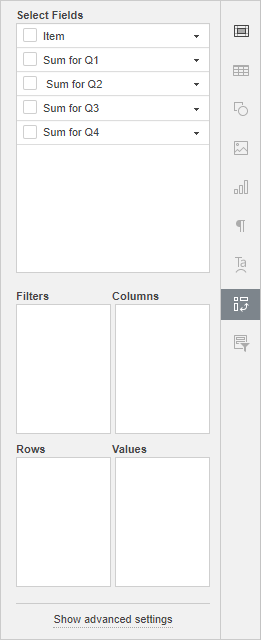
Select fields to display
The Select Fields section contains the fields named according to the column headers in your source data set. Each field contains values from the corresponding column of the source table. The following four sections are available below: Filters, Columns, Rows, and Values.
Check the fields you want to display in the pivot table. When you check a field, it will be added to one of the available sections on the right sidebar depending on the data type and will be displayed in the pivot table. Fields containing text values will be added to the Rows section; fields containing numeric values will be added to the Values section.
You can simply drag fields to the necessary section as well as drag the fields between sections to quickly reorganize your pivot table. To remove a field from the current section, drag it out of this section.
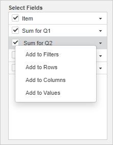
In order to add a field to the necessary section, it's also possible to click the black arrow to the right of a field in the Select Fields section and choose the necessary option from the menu: Add to Filters, Add to Rows, Add to Columns, Add to Values.
Below you can see some examples of using the Filters, Columns, Rows, and Values sections.
-
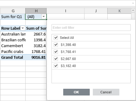
If you add a field to the Filters section, a separate filter will be added above the pivot table. It will be applied to the entire pivot table. If you click the drop-down arrow in the added filter, you'll see the values from the selected field. When you uncheck some values in the filter option window and click OK, the unchecked values will not be displayed in the pivot table.
-
If you add a field to the Columns section, the pivot table will contain a number of columns equal to the number of values from the selected field. The Grand Total column will also be added.
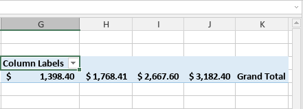
-
If you add a field to the Rows section, the pivot table will contain a number of rows equal to the number of values from the selected field. The Grand Total row will also be added.
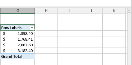
-
If you add a field to the Values section, the pivot table will display the summation value for all numeric values from the selected field. If the field contains text values, the count of values will be displayed. The function used to calculate the summation value can be changed in the field settings.

To see more information regarding any value field, click it with the right mouse button to open the context menu and choose the Show details option, or double click the required value field with the left mouse button. The data that the value field is based on will open in a new sheet.
Rearrange fields and adjust their properties
Once the fields are added to the necessary sections, you can manage them to change the layout and format of the pivot table. Click the black arrow to the right of a field within the Filters, Columns, Rows, or Values sections to access the field context menu.
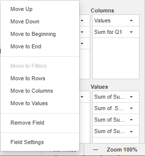
It allows you to:
- Move the selected field Up, Down, to the Beginning, or to the End of the current section if you have added more than one field to the current section.
- Move the selected field to a different section - to Filters, Columns, Rows, or Values. The option that corresponds to the current section will be disabled.
- Remove the selected field from the current section.
- Adjust the selected field settings.
The Filters, Columns, and Rows field settings look similarly:
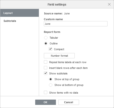
The Layout tab contains the following options:
- The Source name option allows you to view the field name corresponding to the column header from the source data set.
- The Custom name option allows you to change the name of the selected field displayed in the pivot table.
-
The Report Form section allows you to change the way the selected field is displayed in the pivot table:
-
Choose the necessary layout for the selected field in the pivot table:
-
The Tabular form displays one column for each field and provides space for field headers.
-
The Outline form displays one column for each field and provides space for field headers. It also allows you to display subtotals at the top of groups.
-
The Compact form displays items from different row section fields in a single column.
- The Number format option allows you to choose the required number format for the value field. Click this button, choose the required format from the Category list, then click OK when ready. To learn more about number formats, please refer to the following article.
- The Repeat items labels at each row option allows you to visually group rows or columns together if you have multiple fields in the tabular form.
- The Insert blank rows after each item option allows you to add blank lines after items of the selected field.
- The Show subtotals option allows you to choose if you want to display subtotals for the selected field. You can select one of the options: Show at top of group or Show at bottom of group.
- The Show items with no data option allows you to show or hide blank items in the selected field.
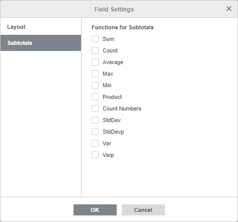
The Subtotals tab allows you to choose Functions for Subtotals. Check the necessary functions in the list: Sum, Count, Average, Max, Min, Product, Count Numbers, StdDev, StdDevp, Var, Varp.
Values field settings
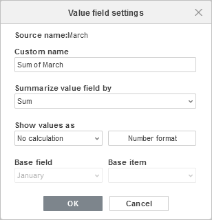
- The Source name option allows you to view the field name corresponding to the column header from the source data set.
- The Custom name option allows you to change the name of the selected field displayed in the pivot table.
- The Summarize value field by option allows you to choose the function used to calculate the summation value for all values from this field. By default, Sum is used for numeric values, Count is used for text values. The available functions are Sum, Count, Average, Max, Min, Product, Count Numbers, StdDev, StdDevp, Var, Varp.
- The Show values as option allows you to show instant custom calculations instead of adding a formula and creating a calculated field. No calculation is the default option that displays the actual value in the field. Other calculation options: % of grand total, % of column total, % of row total, % of, % of parent row total, % of parent column total, % of parent total, Difference from, % difference from, Running total in, % running total in, Rank smallest to largest, Rank largest to smallest, Index. Use Base field and Base item when these options are available for the calculation you selected (% of, % of parent total, Difference from, % difference from, Running total in, % running total in).
- The Number format option allows you to choose the required number format for the value field. Click this button, choose the required format from the Category list, then click OK when ready. To learn more about number formats, please refer to the following article.
Group and ungroup data
Data in pivot tables can be grouped according to custom requirements. Grouping is available for dates and basic numbers.
Grouping dates
To group dates, create a pivot table incorporating a set of needed dates. Right click any cell in a pivot table with a date, choose the Group option in the pop-up menu, and set the needed parameters in the opened window.
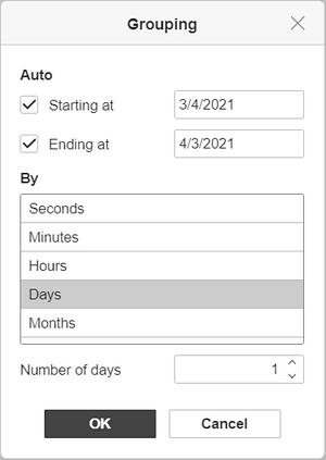
- Starting at - the first date in the source data is chosen by default. To change it, enter the needed date in this field. Deactivate this box to ignore the starting point.
- Ending at - the last date in the source data is chosen by default. To change it, enter the needed date in this field. Deactivate this box to ignore the ending point.
- By - the Seconds, Minutes, and Hours options group the data according to the time given in the source data. The Months option eliminates days and leaves months only. The Quarters option operates at a condition: four months constitute a quarter, thus providing Qtr1, Qtr2, etc. The Years option groups dates as per years given in the source data. Combine the options to achieve the needed result.
- Number of days - set the required value to determine a date range.
- Click OK when finished.
Grouping numbers
To group numbers, create a pivot table incorporating a set of needed numbers. Right click any cell in a pivot table with a number, choose the Group option in the pop-up menu, and set the needed parameters in the opened window.
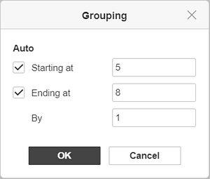
- Starting at - the smallest number in the source data is chosen by default. To change it, enter the needed number in this field. Deactivate this box to ignore the smallest number.
- Ending at - the largest number in the source data is chosen by default. To change it, enter the needed number in this field. Deactivate this box to ignore the largest number.
- By - set the required interval for grouping numbers. E.g., “2” will group the set of numbers from 1 through 10 as “1-2”, “3-4”, etc.
- Click OK when finished.
Ungrouping data
To ungroup previously grouped data,
- right-click any cell that is in the group,
- select the Ungroup option in the context menu.
Change the appearance of pivot tables
You can use options available on the top toolbar to adjust the way your pivot table is displayed. These options are applied to the entire pivot table.
Select at least one cell within the pivot table with the mouse to activate the editing tools on the top toolbar.

The Select button allows you to select the entire pivot table.
If you change the data in your source data set, select the pivot table and click the Refresh button to update the pivot table.
Expand or collapse fields
To expand or collapse data details, click a field with the right mouse button to open the context menu, choose the Expand/Collapse menu item, then select the necessary option:
- Expand - to show details for the currently selected item.
- Collapse - to hide details for the currently selected item.
- Expand Entire Field - to show details for all items in a field. The similar setting is also available at the top toolbar.
- Collapse Entire Field - to hide details for all items in a field. The similar setting is also available at the top toolbar.
The groups are hidden behind the plus/minus icons. You can also expand/collapse fields by double-clicking the pivot table headers.
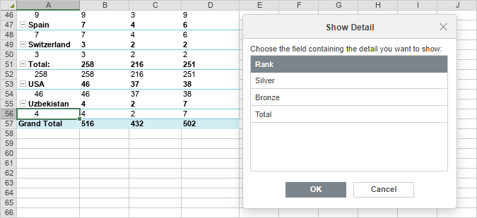
The Expand option, when the last field of rows or columns is selected, opens a dialog window for adding a new field to the row or column. Choose the necessary field and click OK.
Change the style of pivot tables
You can change the appearance of pivot tables in a spreadsheet using the style editing tools available on the top toolbar.
Select at least one cell within the pivot table with the mouse to activate the editing tools on the top toolbar.

The rows and columns options allow you to emphasize certain rows/columns applying specific formatting to them, or highlight different rows/columns with different background colors to clearly distinguish them. The following options are available:
- Row Headers - allows you to highlight the row headers with special formatting.
- Column Headers - allows you to highlight the column headers with special formatting.
- Banded Rows - enables the background color alternation for odd and even rows.
- Banded Columns - enables the background color alternation for odd and even columns.
The template list allows you to choose one of the predefined pivot table styles. Each template combines certain formatting parameters, such as a background color, border style, row/column banding, etc.
Depending on the options checked for rows and columns, the templates set will be displayed differently. For example, if you've checked the Row Headers and Banded Columns options, the visible part of the templates list will include templates with the row headers highlighted and banded columns enabled, but you can expand the full list by clicking the arrow to see all the available templates.
Filter, sort and add slicers in pivot tables
You can filter pivot tables by labels or values and use the additional sort parameters.
Filtering
Click the drop-down arrow in the Row Labels or Column Labels of the pivot table. The Filter option list will open:
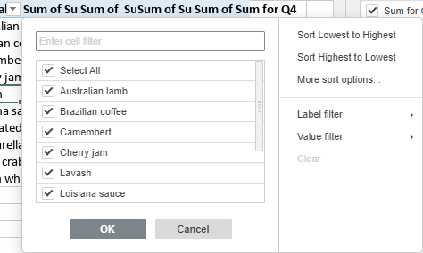
Adjust the filter parameters. You can proceed in one of the following ways: select the data to display or filter the data by certain criteria.
-
Select the data to display
Uncheck the boxes near the data you need to hide. For your convenience, all the data within the Filter option list are sorted in ascending order.
Note: the (blank) checkbox corresponds to the empty cells. It is available if the selected cell range contains at least one empty cell.
To facilitate the process, make use of the search field on the top. Enter your query, entirely or partially, in the field - the values that include these characters will be displayed in the list below. The following two options will be also available:
- Select All Search Results - is checked by default. It allows selecting all the values that correspond to your query in the list.
- Add current selection to filter - if you check this box, the selected values will not be hidden when you apply the filter.
After you select all the necessary data, click the OK button in the Filter option list to apply the filter.
-
Filter data by certain criteria
You can choose either the Label filter or the Value filter option on the right side of the Filter options list, and then select one of the options from the submenu:
-
For the Label filter the following options are available:
- For texts: Equals..., Does not equal..., Begins with..., Does not begin with..., Ends with..., Does not end with..., Contains..., Does not contain...
- For numbers: Greater than..., Greater than or equal to..., Less than..., Less than or equal to..., Between, Not between.
- For the Value filter the following options are available: Equals..., Does not equal..., Greater than..., Greater than or equal to..., Less than..., Less than or equal to..., Between, Not between, Top 10.
After you select one of the above options (apart from Top 10), the Label/Value Filter window will open. The corresponding field and criterion will be selected in the first and second drop-down lists. Enter the necessary value in the field on the right.
Click OK to apply the filter.
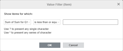
If you choose the Top 10 option from the Value filter option list, a new window will open:
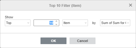
The first drop-down list allows choosing if you wish to display the highest (Top) or the lowest (Bottom) values. The second field allows specifying how many entries from the list or which percent of the overall entries number you want to display (you can enter a number from 1 to 500). The third drop-down list allows setting the units of measure: Item, Percent, or Sum. The fourth drop-down list displays the selected field name. Once the necessary parameters are set, click OK to apply the filter.
The Filter button will appear in the Row Labels or Column Labels of the pivot table. It means that the filter is applied.
Sorting
You can sort your pivot table data using the sort options. Click the drop-down arrow in the Row Labels or Column Labels of the pivot table and then select Sort Lowest to Highest or Sort Highest to Lowest option from the submenu.
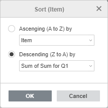
The More Sort Options option allows you to open the Sort window where you can select the necessary sorting order - Ascending or Descending - and then select a certain field you want to sort.
Adding slicers
You can add slicers to filter data easier by displaying only what is needed. To learn more about slicers, please read the guide on creating slicers.
Adjust pivot table advanced settings
To change the advanced settings of the pivot table, use the Show advanced settings link on the right sidebar. The 'Pivot Table - Advanced Settings' window will open:
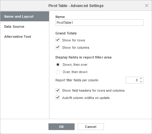
The Name and Layout tab allows you to change the pivot table common properties.
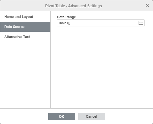
The Data Source tab allows you to change the data you wish to use to create the pivot table.
Check the selected Data Range and modify it, if necessary. To do that, click the icon.
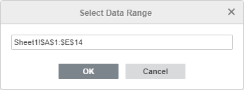
In the Select Data Range window, enter the necessary data range in the following format: Sheet1!$A$1:$E$10. You can also select the necessary cell range in the sheet using the mouse. When ready, click OK.
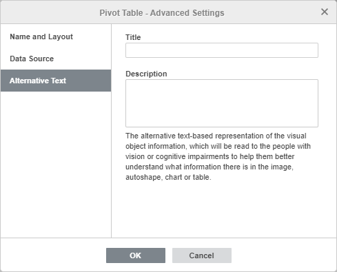
The Alternative Text tab allows specifying the Title and the Description which will be read to people with vision or cognitive impairments to help them better understand what information the pivot table contains.
Delete a pivot table
To delete a pivot table,
- Select the entire pivot table using the Select button on the top toolbar.
- Press the Delete key.
Calculated items
Calculated items are used for basic calculations between different items within a single field.
To add a calculated item:
- Select the required field.
- Go to the Pivot Table tab and click the Calculated Items button on the top toolbar.
-
Enter the Item Name, which will be displayed as a pivot table field name later.
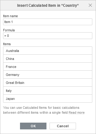
- Edit the Formula field by typing in the required fields from the list below or by clicking the plus button to the right of them, and entering the required mathematical symbols, e.g., "+" or "-".
-
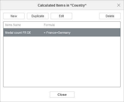
Click OK. To further manage created calculated items, use the corresponding buttons at the top of the window: add a new one, duplicated, edit, or delete the currently selected one.
Return to previous page