Freezing rows and columns in ONLYOFFICE Spreadsheet Editor

Select the cell located below the row you want to lock and to the right of the column you want to lock.

Here you can see a number of simple examples explaining which cell, row or column should be selected to freeze certain rows or columns or both rows and columns at once:

• To lock the top-most row only, select cell A2 / the entire row 2, or use the Freeze Top Row option available in the Freeze Panes drop-down menu on the View tab,
• To freeze multiple rows on the top, select the row below the last row you want to lock,
• To lock the left-most column only, select cell B1 / the entire column B, or use the Freeze First Column option available in the Freeze Panes drop-down menu on the View tab,
• To freeze multiple columns on the left, select the column to the right of the last column you want to lock,
• To freeze the first column and the top row of the worksheet simultaneously, select cell B2,
• To freeze two rows on the top and two columns on the left at the same time, select cell C3.

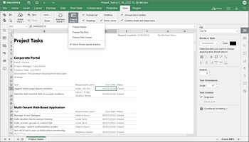
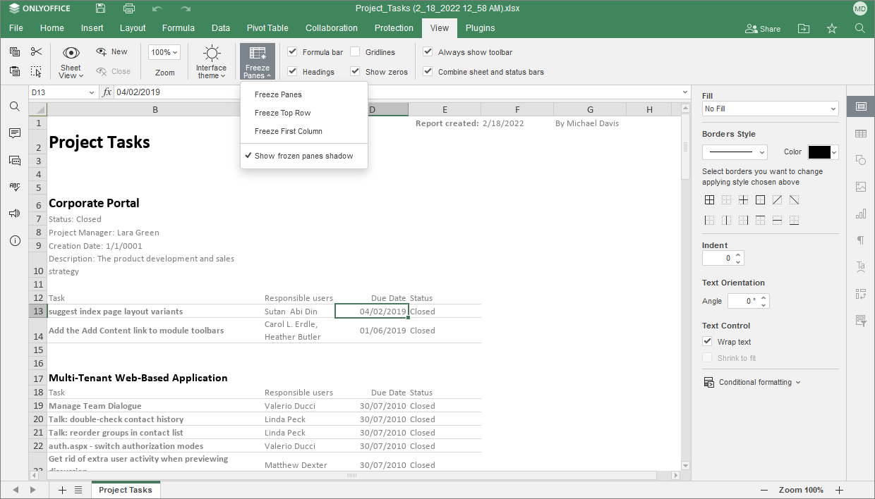
Click the View settings icon in the upper right corner of the top toolbar, or go to the View tab, or right-click the selected cell to open the contextual menu. Select the Freeze Panes option in the menu and choose one of the available presets: Freeze Panes (depends on the previously selected cell), Freeze Top Row, and Freeze First Column.

By default, a subtle green line shows where a frozen column and/or rows starts. To disable or enable it, go to View tab, click the Freeze Pane button, and click Show frozen panes shadow. The Show frozen panes shadow option is also available on the View settings menu on the right side of the top toolbar.

When the Show frozen panes shadow is disabled, a horizontal or vertical gray line shows the frozen columns or lines. The areas above and to the left of these lines are locked. Now you can scroll your worksheet to make sure that all the necessary data remain visible.

To unlock the previously frozen rows and columns, just open the View settings menu and click the Freeze Panes option once again, or right-click anywhere within the worksheet and select the Unfreeze Panes option from the context menu, or go to the View tab, click the Freeze Panes button and select the Unfreeze Panes option.